Vignette for Jaya, an R package for gradient-free Jaya optimization algorithm
This post is a demonstration for Jaya, an R package for gradient-free Jaya optimization algorithm.
In the year 2015, Prof. R. Venkata Rao from Sardar Vallabhbhai National Institute of Technology Surat, India proposed and published the Jaya optimization algorithm, which is now among the popular ones for solving constrained and unconstrained optimization problems. This algorithm has now solved several real-life problems. In the year 2019, we (Mr. Mayur Kishor Shende and I) developed an R package for this algorithm, named Jaya. In this article, I have discussed the vignette of the package and demonstrated how to use this package. The official webpage for the Jaya package is https://cran.r-project.org/package=Jaya, and it can be cited as Mayur Shende and Neeraj Bokde (2019). Jaya: Jaya, a Gradient-Free Optimization Algorithm. R package version 0.1.9. https://CRAN.R-project.org/package=Jaya
Jaya Algorithm (JA)
Jaya Algorithm is a gradient-free optimization algorithm [1]. It can be used for Maximization or Minimization of a function. It is a population based method which repeatedly modifies a population of individual solutions and capable of solving both constrained and unconstrained optimization problems. It does not contain any hyperparameters. Following examples demonstrate the performance of Jaya package. The examples are selected from the well-known report [2].
Demonstration of Jaya package:
Load Jaya package.
library(Jaya)

## Warning: pakke 'Jaya' blev bygget under R version 4.1.3
Unconstrainted Problem
Minimize,
subject to,
− 100 ≤ xi ≤ 100
# Test Function to minimize
square <- function(x){
return((x[1]*x[1])+(x[2]*x[2]))
}
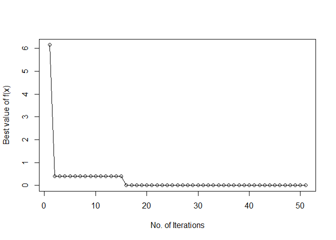
a <- jaya(fun = square, lower = c(-100,-100), upper = c(100,100), maxiter = 50, n_var = 2, seed = 100)
## function(x){
## return((x[1]*x[1])+(x[2]*x[2]))
## }
## <bytecode: 0x0000000016aad0d8>
## x1 x2 f(x)
## Best -0.0004926281 0.0002143597 2.886326e-07
summary(a)
## Jaya Algorithm
## Population Size = 50
## Number of iterations = 50
## Number of variables = 2
##
## MINIMIZE,
## function(x){
## return((x[1]*x[1])+(x[2]*x[2]))
## }
## <bytecode: 0x0000000016aad0d8>
##
## Limits:
## x1 = [-100,100]
## x2 = [-100,100]
##
## Best Result:
## x1 x2 f(x)
## Best -0.0004926281 0.0002143597 2.886326e-07
## Suggestions for the initial population:
## dataramme med 0 kolonner og 0 rækker
plot(a)
Constrainted Problem
g24 (Source: [2])
Minimize, f(x) = − x1 − x2
subject to,
g24 <- function(x)
{
f <- f(x)
pen1 <- max(0, c1(x))
pen2 <- max(0, c2(x))
return(f + pen1 + pen2)
}
f <- function(x)
{ return(-x[1]-x[2]) }
#Constraints
c1 <- function(x)
{ return( -2*(x[1]**4) + 8*(x[1]**3) - 8*(x[1]**2) + x[2] - 2 ) }
c2 <- function(x)
{ return( -4*(x[1]**4) + 32*(x[1]**3) - 88*(x[1]**2) + 96*x[1] + x[2] -36 ) }
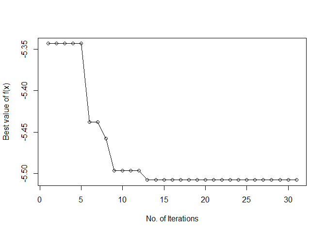
b <- jaya(fun = g24, lower = c(0,0), upper = c(3,4), popSize = 30, maxiter = 30, n_var = 2, seed = 100)
## function(x)
## {
## f <- f(x)
## pen1 <- max(0, c1(x))
## pen2 <- max(0, c2(x))
## return(f + pen1 + pen2)
## }
## <bytecode: 0x000000001c49a500>
## x1 x2 f(x)
## Best 2.329554 3.178352 -5.507887
summary(b)
## Jaya Algorithm
## Population Size = 30
## Number of iterations = 30
## Number of variables = 2
##
## MINIMIZE,
## function(x)
## {
## f <- f(x)
## pen1 <- max(0, c1(x))
## pen2 <- max(0, c2(x))
## return(f + pen1 + pen2)
## }
## <bytecode: 0x000000001c49a500>
##
## Limits:
## x1 = [0,3]
## x2 = [0,4]
##
## Best Result:
## x1 x2 f(x)
## Best 2.329554 3.178352 -5.507887
## Suggestions for the initial population:
## dataramme med 0 kolonner og 0 rækker
plot(b)
g11 (Source: [2])
Minimize, f(x) = x12 + (x2 − 1)2
subject to,
# Test Function to minimize
g11 <- function(x)
{
f <- f(x)
if(round(c1(x),2) != 0){
return(f + c1(x))
}
return(f)
}
f <- function(x)
{ return(x[1]**2 + (x[2] - 1)**2) }
c1 <- function(x)
{ return(x[2] - x[1]**2) }
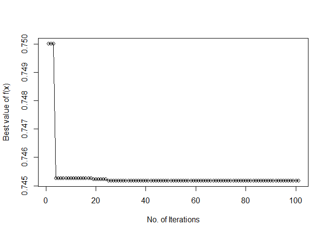
c <- jaya(fun = g11, lower = c(-1,-1), upper = c(1,1), maxiter = 100, n_var = 2, seed = 100)
## function(x)
## {
## f <- f(x)
## if(round(c1(x),2) != 0){
## return(f + c1(x))
## }
## return(f)
## }
## <bytecode: 0x0000000016324bd8>
## x1 x2 f(x)
## Best 0.708031 0.5061709 0.745175
summary(c)
## Jaya Algorithm
## Population Size = 50
## Number of iterations = 100
## Number of variables = 2
##
## MINIMIZE,
## function(x)
## {
## f <- f(x)
## if(round(c1(x),2) != 0){
## return(f + c1(x))
## }
## return(f)
## }
## <bytecode: 0x0000000016324bd8>
##
## Limits:
## x1 = [-1,1]
## x2 = [-1,1]
##
## Best Result:
## x1 x2 f(x)
## Best 0.708031 0.5061709 0.745175
## Suggestions for the initial population:
## dataramme med 0 kolonner og 0 rækker
plot(c)
Comparison with Genetic Algorithm (GA):
This section compares the performance of JA with GA for a contrained function discussed in [1]. For comparison purpose R package GA [3] is used.
Minimize, f(x) = 100(x12 − x2)2 + (1 − x2)2
subject to,
# Function to test for
f <- function(x)
{ return( 100*((x[1]**2 - x[2])**2) + (1 - x[1])**2 ) }

# Constraints
c1 <- function(x)
{ return( (x[1]*x[2]) + x[1] - x[2] + 1.5) }

c2 <- function(x)
{ return(10 - (x[1]*x[2])) }

# Function with penalty
con <- function(x){
  func <- -f(x)
  pen <- sqrt(.Machine$double.xmax)
  pen1 <- max(0, c1(x))*pen
  pen2 <- max(0, c2(x))*pen
  return(func - pen1 - pen2)
}
For GA,
library(GA)
G <- ga("real-valued", fitness = con, lower = c(0,0), upper = c(1,13),
         maxiter = 1000, run = 200, seed = 123)
# Values of x1 and x2
G@solution

##             x1       x2
## [1,] 0.8120632 12.31468

# Value of f(x)
G@fitnessValue

## [1] -13584.49
For JA,
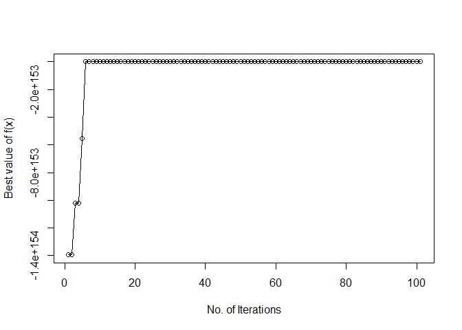
d <- jaya(fun = con, lower = c(0,0),  upper = c(1,13), maxiter = 100, n_var = 2, seed = 123, opt = "Maximize")

## function(x){
##   func <- -f(x)
##   pen <- sqrt(.Machine$double.xmax)
##   pen1 <- max(0, c1(x))*pen
##   pen2 <- max(0, c2(x))*pen
##   return(func - pen1 - pen2)
## }
## <bytecode: 0x000000001c9810d8>
##             x1      x2      f(x)
## Best 0.8122023 12.3122 -13578.18

summary(d)

## Jaya Algorithm
## Population Size      =  50
## Number of iterations =  100
## Number of variables  =  2
##
## MAXIMIZE,
## function(x){
##   func <- -f(x)
##   pen <- sqrt(.Machine$double.xmax)
##   pen1 <- max(0, c1(x))*pen
##   pen2 <- max(0, c2(x))*pen
##   return(func - pen1 - pen2)
## }
## <bytecode: 0x000000001c9810d8>
##
## Limits:
## x1 = [0,1]
## x2 = [0,13]
##
## Best Result:
##             x1      x2      f(x)
## Best 0.8122023 12.3122 -13578.18
## Suggestions for the initial population:
## dataramme med 0 kolonner og 0 rækker

plot(d)
References
[1] Rao, R. (2016). Jaya: A simple and new optimization algorithm for solving constrained and unconstrained optimization problems. International Journal of Industrial Engineering Computations, 7(1), 19-34.
[2] Liang, J. J., Runarsson, T. P., Mezura-Montes, E., Clerc, M., Suganthan, P. N., Coello, C. C., & Deb, K. (2006). Problem definitions and evaluation criteria for the CEC 2006 special session on constrained real-parameter optimization. Journal of Applied Mechanics, 41(8), 8-31.
[3] Scrucca, L. (2013). GA: a package for genetic algorithms in R. Journal of Statistical Software, 53(4), 1-37.