Vignette for ForecastTB, an R package as a testbench for time series forecasting
This post is a demonstration for ForecastTB, an R package as a testbench for time series forecasting.
The ForecastTB is a plug-and-play structured module, and several forecasting methods can be included with simple instructions. This test-bench is not limited to the default forecasting and error metric functions, and users are able to append, remove, or choose the desired methods as per requirements. Besides, several plotting functions and statistical performance metrics are provided in this package to visualize the comparative performance and accuracy of different forecasting methods. This package is available on CRAN (https://cran.r-project.org/package=ForecastTB) and its published article is: Bokde, N.D.; Yaseen, Z.M.; Andersen, G.B. ForecastTB—An R Package as a Test-Bench for Time Series Forecasting—Application of Wind Speed and Solar Radiation Modeling. Energies 2020, 13, 2578. https://doi.org/10.3390/en13102578.
Demonstration of ‘ForecastTB’ package:
This document demonstates the R package ‘ForecastTB’. It is intended for comparing the performance of forecasting methods. The package assists in developing background, strategies, policies and environment needed for comparison of forecasting methods. A comparison report for the defined framework is produced as an output. Load the package as following:
library(ForecastTB)

## Warning: pakke 'ForecastTB' blev bygget under R version 4.1.3

## Registered S3 method overwritten by 'quantmod':
##   method            from
##   as.zoo.data.frame zoo
The basic function of the package is prediction_errors(). Following are the parameters considered by this function:
data: input time series for testingnval: an integer to decide number of values to predict (default:12)ePara: type of error calculation (RMSE and MAE are default), add an error parameter of your choice in the following manner:ePara = c("errorparametername"), where errorparametername is should be a source/function which returns desired error set. (default:RMSEandMAE)ePara_name: list of names of error parameters passed in order (default:RMSEandMAE)Method: list of locations of function for the proposed prediction method (should be recursive) (default:ARIMA)MethodName: list of names for function for the proposed prediction method in order (default:ARIMA)strats: list of forecasting strategies. Available :recursiveanddirRec. (default:recursive)append_: suggests if the function is used to append to another instance. (default:1)dval: last d values of the data to be used for forecasting (default: length of thedata)
The prediction_errors() function returns, two slots as output. First slot is output, which provides Error_Parameters, indicating error values for the forecasting methods and error parameters defined in the framework, and Predicted_Values as values forecasted with the same foreasting methods. Further, the second slot is parameters, which returns the parameters used or provided to prediction_errors() function.
a <- prediction_errors(data = nottem)  #`nottem` is a sample dataset in CRAN

a

## An object of class "prediction_errors"
## Slot "output":
## $Error_Parameters
##           RMSE      MAE     MAPE exec_time
## ARIMA 2.340092 1.932982 4.215609  0.828805
##
## $Predicted_Values
##                    1        2        3        4        5        6        7
## Test values 39.40000 40.90000 42.40000 47.80000 52.40000 58.00000 60.70000
## ARIMA       37.41933 37.69716 41.18252 46.29926 52.24804 57.10696 59.71674
##                    8        9      10       11       12
## Test values 61.80000 58.20000 46.7000 46.60000 37.80000
## ARIMA       59.41173 56.38197 51.4756 46.04203 41.52592
##
##
## Slot "parameters":
## $data
##       Jan  Feb  Mar  Apr  May  Jun  Jul  Aug  Sep  Oct  Nov  Dec
## 1920 40.6 40.8 44.4 46.7 54.1 58.5 57.7 56.4 54.3 50.5 42.9 39.8
## 1921 44.2 39.8 45.1 47.0 54.1 58.7 66.3 59.9 57.0 54.2 39.7 42.8
## 1922 37.5 38.7 39.5 42.1 55.7 57.8 56.8 54.3 54.3 47.1 41.8 41.7
## 1923 41.8 40.1 42.9 45.8 49.2 52.7 64.2 59.6 54.4 49.2 36.3 37.6
## 1924 39.3 37.5 38.3 45.5 53.2 57.7 60.8 58.2 56.4 49.8 44.4 43.6
## 1925 40.0 40.5 40.8 45.1 53.8 59.4 63.5 61.0 53.0 50.0 38.1 36.3
## 1926 39.2 43.4 43.4 48.9 50.6 56.8 62.5 62.0 57.5 46.7 41.6 39.8
## 1927 39.4 38.5 45.3 47.1 51.7 55.0 60.4 60.5 54.7 50.3 42.3 35.2
## 1928 40.8 41.1 42.8 47.3 50.9 56.4 62.2 60.5 55.4 50.2 43.0 37.3
## 1929 34.8 31.3 41.0 43.9 53.1 56.9 62.5 60.3 59.8 49.2 42.9 41.9
## 1930 41.6 37.1 41.2 46.9 51.2 60.4 60.1 61.6 57.0 50.9 43.0 38.8
## 1931 37.1 38.4 38.4 46.5 53.5 58.4 60.6 58.2 53.8 46.6 45.5 40.6
## 1932 42.4 38.4 40.3 44.6 50.9 57.0 62.1 63.5 56.3 47.3 43.6 41.8
## 1933 36.2 39.3 44.5 48.7 54.2 60.8 65.5 64.9 60.1 50.2 42.1 35.8
## 1934 39.4 38.2 40.4 46.9 53.4 59.6 66.5 60.4 59.2 51.2 42.8 45.8
## 1935 40.0 42.6 43.5 47.1 50.0 60.5 64.6 64.0 56.8 48.6 44.2 36.4
## 1936 37.3 35.0 44.0 43.9 52.7 58.6 60.0 61.1 58.1 49.6 41.6 41.3
## 1937 40.8 41.0 38.4 47.4 54.1 58.6 61.4 61.8 56.3 50.9 41.4 37.1
## 1938 42.1 41.2 47.3 46.6 52.4 59.0 59.6 60.4 57.0 50.7 47.8 39.2
## 1939 39.4 40.9 42.4 47.8 52.4 58.0 60.7 61.8 58.2 46.7 46.6 37.8
##
## $nval
## [1] 12
##
## $ePara
## [1] "RMSE" "MAE"  "MAPE"
##
## $ePara_name
## [1] "RMSE" "MAE"  "MAPE"
##
## $Method
## [1] "ARIMA"
##
## $MethodName
## [1] "ARIMA"
##
## $Strategy
## [1] "Recursive"
##
## $dval
## [1] 240
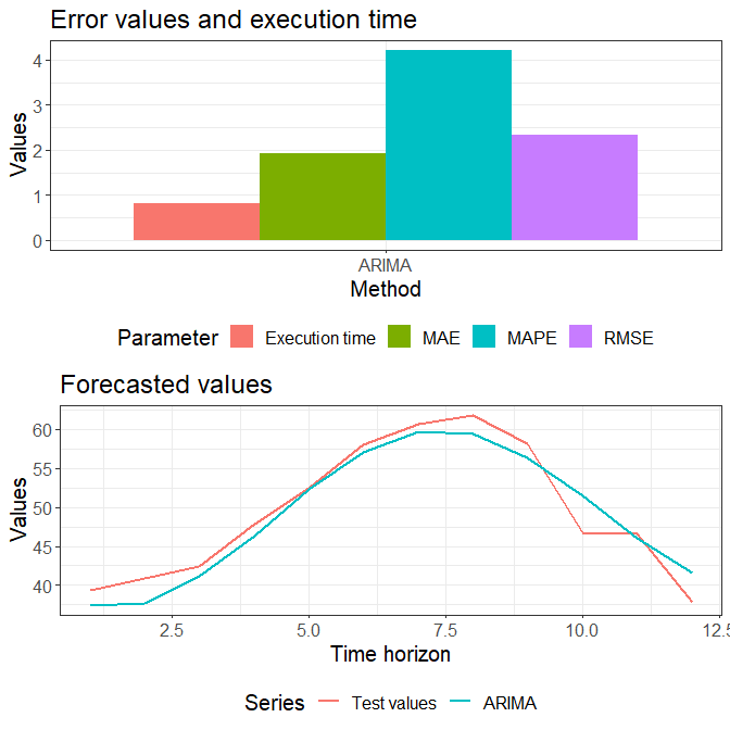
The quick visualization of the object retuned with prediction_errors() function can be done with plot() function as below:
b <- plot(a)
Comparison of multiple methods:
As discussed above, prediction_errors() function evaluates the performance of ARIMA method. In addition, it allows to compare performance of distinct methods along with ARIMA. In following example, two methods (LPSF and PSF) are compared along with the ARIMA. These methods are formatted in the form of a function, which requires data and nval as input parameters and must return the nval number of frecasted values as a vector. In following code, test1() and test2() functions are used for LPSF and PSF methods, respectively.
library(decomposedPSF)

## Warning: pakke 'decomposedPSF' blev bygget under R version 4.1.3

test1 <- function(data, nval){
   return(lpsf(data = data, n.ahead = nval))
}

library(PSF)

## Warning: pakke 'PSF' blev bygget under R version 4.1.3

test2 <- function(data, nval){
  a <- psf(data = data, cycle = 12)
  b <- predict(object = a, n.ahead = nval)
  return(b)
}
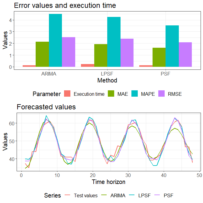
Following code chunk show how user can attach various methods in the prediction_errors() function. In this chunk, the append_ parameter is assigned 1, to appned the new methods (LPSF and PSF) in addition to the default ARIMA method. On contrary, if the append_parameter is assigned 0, only newly added LPSF and PSF nethods would be compared.
a1 <- prediction_errors(data = nottem, nval = 48,
                        Method = c("test1(data, nval)", "test2(data, nval)"),
                        MethodName = c("LPSF","PSF"), append_ = 1)
a1@output$Error_Parameters

##            RMSE       MAE      MAPE exec_time
## ARIMA 2.5233156 2.1280641 4.5135378 0.1318271
## LPSF  2.3915796 1.9361111 4.2386499 0.2356999
## PSF   2.0891640 1.6273176 3.5196094 0.1198409

b1 <- plot(a1)
Appending new methods:
Consider, another function test3(), which is to be added to an already existing object prediction_errors, eg. a1.
library(forecast)
test3 <- function(data, nval){
  b <- as.numeric(forecast(ets(data), h = nval)$mean)
  return(b)
}
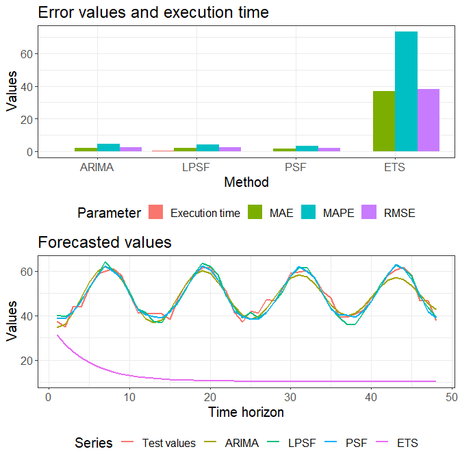
For this purpose, the append_() function can be used as follows:
The append_() function have object, Method, MethodName, ePara and ePara_name parameters, with similar meaning as that of used in prediction_errors() function. Other hidden parameters of the append_() function automatically get synced with the prediction_errors() function.
c1 <- append_(object = a1, Method = c("test3(data,nval)"), MethodName = c('ETS'))
c1@output$Error_Parameters

##              RMSE         MAE        MAPE   exec_time
## ARIMA   2.5233156   2.1280641   4.5135378   0.1318271
## LPSF    2.3915796   1.9361111   4.2386499   0.2356999
## PSF     2.0891640   1.6273176   3.5196094   0.1198409
## ETS   38.29743056 36.85216463 73.47667823  0.04393792

d1 <- plot(c1)
Removing methods:
When more than one methods are established in the environment and the user wish to remove one or more of these methods from it, the choose_() function can be used. This function takes a prediction_errors object as input shows all methods established in the environment, and asks the number of methods which the user wants to remove from it.
In the following example, the user supplied 4 as input, which reflects Method 4: ETS, and in response to this, the choose_() function provides a new object with updated method lists.
# > e1 <- choose_(object = c1)
# Following are the methods attached with the object:
#         [,1]    [,2]   [,3]  [,4]
# Indices "1"     "2"    "3"   "4"
# Methods "ARIMA" "LPSF" "PSF" "ETS"
#
# Enter the indices of methods to remove:4
#
# > e1@output$Error_Parameters
#            RMSE       MAE exec_time
# ARIMA 2.5233156 2.1280641 0.1963789
# LPSF  2.3915796 1.9361111 0.2990961
# PSF   2.2748736 1.8301389 0.1226711
Adding new Error metrics:
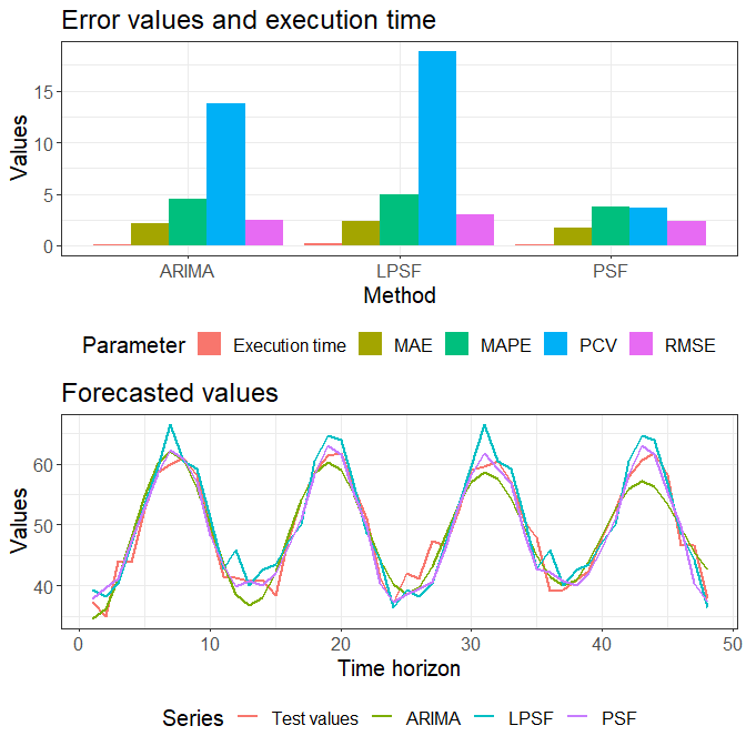
In default scenario, the prediction_errors() function compares forecasting methods in terms of RMSE, MAE and MAPE. In addition, it allows to append multiple new error metrics. The Percent change in variance (PCV) is an another error metric with following definition:
where var(Predicted) and var(Observed) are variance of predicted and obvserved values. Following chunk code is the function for PCV error metric:
pcv <- function(obs, pred){
  d <- (var(obs) - var(pred)) * 100/ var(obs)
  d <- abs(as.numeric(d))
  return(d)
}
Following chunk code is used to append PCV as a new error metric in existing prediction_errors object.
a1 <- prediction_errors(data = nottem, nval = 48,
                        Method = c("test1(data, nval)", "test2(data, nval)"),
                        MethodName = c("LPSF","PSF"),
                        ePara = "pcv(obs, pred)", ePara_name = 'PCV',
                        append_ = 1)
a1@output$Error_Parameters

##             RMSE        MAE       MAPE        PCV  exec_time
## ARIMA  2.5233156  2.1280641  4.5135378 13.7570726  0.1118529
## LPSF    2.964653   2.345833   4.930034  18.849908   0.235734
## PSF    2.3423919  1.7383333  3.7365227  3.6103638  0.1038711

b1 <- plot(a1)
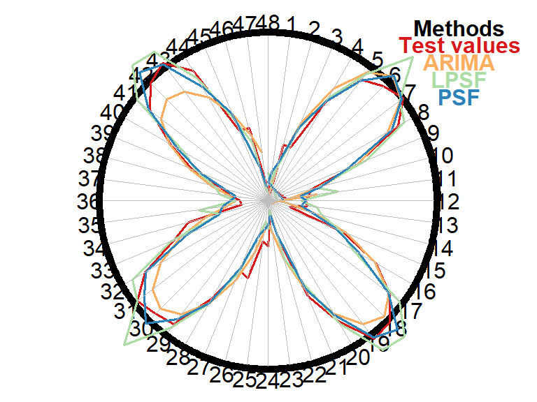
A unique plot:
A unique way of showing forecasted values, especially if these are seasonal values, the following function can be used. This plot shows how forecatsed observations are behaving on an increasing number of seasonal time horizons.
plot_circle(a1)

## `major.tick.percentage` is not used any more, please directly use argument `major.tick.length`.

## Note: 48 points are out of plotting region in sector 'a', track '1'.
Monte-Carlo strategy:
Monte-Carlo is a popular strategy to compare the performance of forecasting methods, which selects multiple patches of dataset randomly and test performance of forecasting methods and returns the average error values.
The Monte-Carlo strategy ensures an accurate comparison of forecasting methods and avoids the baised results obtained by chance.
This package provides the monte_carlo() function as follows:
The parameters used in this function are:
object: output of ‘prediction_errors()’ functionsize: volume of time series used in Monte Carlo strategyiteration: number of iterations models to be appliedfval: a flag to view forecasted values in each iteration (default: 0, don’t view values)figs: a flag to view plots for each iteration (default: 0, don’t view plots)
This function returns:
- Error values with provided models in each iteration along with the mean values
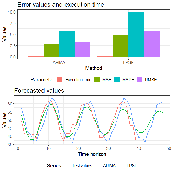
When monte_carlo() function with fval and figs ON flags:
monte_carlo(object = a1, size = 144, iteration = 2, fval = 1, figs = 1)
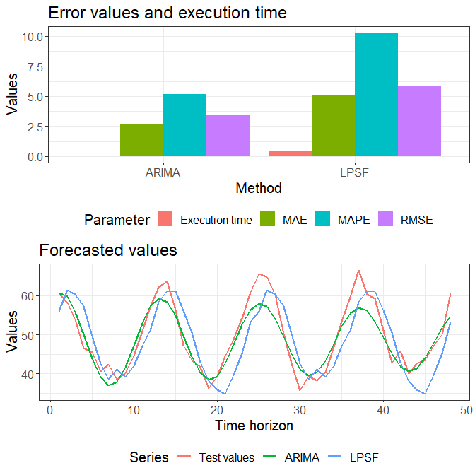
## $Error_Parameters
##         ARIMA     LPSF
## 18   3.447821 5.790689
## 81   3.222167 5.564471
## Mean 3.334994 5.677580
##
## $Predicted_Values
## $Predicted_Values[[1]]
##                    1        2        3        4        5        6        7
## Test values 60.60000 58.20000 53.80000 46.60000 45.50000 40.60000 42.40000
## ARIMA       60.69516 59.77833 55.81699 50.00904 43.93239 39.19682 37.04437
## LPSF        55.95000 61.45000 60.40000 57.25000 49.75000 42.60000 38.55000
##                    8        9       10       11       12       13       14
## Test values 38.40000 40.30000 44.60000 50.90000 57.00000 62.10000 63.50000
## ARIMA       37.99407 41.72755 47.19387 52.90124 57.32446 59.31202 58.38482
## LPSF        41.20000 39.10000 42.00000 47.10000 51.05000 58.40000 61.15000
##                   15      16       17       18       19       20       21
## Test values 56.30000 47.3000 43.60000 41.80000 36.20000 39.30000 44.50000
## ARIMA       54.84994 49.7027 44.34728 40.21435 38.37944 39.28385 42.63015
## LPSF        61.05000 56.2000 50.55000 43.00000 38.05000 35.95000 34.85000
##                  22      23       24       25       26       27       28
## Test values 48.7000 54.2000 60.80000 65.50000 64.90000 60.10000 50.20000
## ARIMA       47.4767 52.5017 56.36311 58.05648 57.17556 54.00809 49.44489
## LPSF        39.7000 45.2000 53.30000 55.95000 61.45000 60.40000 57.25000
##                   29       30       31       32       33       34     35
## Test values 42.10000 35.80000 39.40000 38.20000 40.40000 46.90000 53.400
## ARIMA       44.73012 41.12265 39.56045 40.41738 43.41528 47.71151 52.135
## LPSF        49.75000 42.60000 38.55000 41.20000 39.10000 42.00000 47.100
##                   36       37       38       39       40       41       42
## Test values 59.60000 66.50000 60.40000 59.20000 51.20000 42.80000 45.80000
## ARIMA       55.50498 56.94563 56.11306 53.27593 49.23125 45.08121 41.93331
## LPSF        51.05000 58.40000 61.15000 61.05000 56.20000 50.55000 43.00000
##                   43       44       45       46       47       48
## Test values 40.00000 42.60000 43.50000 47.10000 50.00000 60.50000
## ARIMA       40.60527 41.41326 44.09798 47.90566 51.79898 54.73923
## LPSF        38.05000 35.95000 34.85000 39.70000 45.20000 53.30000
##
## $Predicted_Values[[2]]
##                    1       2        3        4        5        6        7
## Test values 49.60000 41.6000 41.30000 40.80000 41.00000 38.40000 47.40000
## ARIMA       52.75155 46.6133 41.28005 38.14674 37.97027 40.72038 45.59506
## LPSF        57.30000 50.7000 42.90000 41.55000 37.40000 36.95000 42.25000
##                    8        9       10       11       12       13       14
## Test values 54.10000 58.60000 61.40000 61.80000 56.30000 50.90000 41.40000
## ARIMA       51.25767 56.19988 59.14332 59.36876 56.89004 52.43071 47.21498
## LPSF        45.50000 51.55000 58.70000 63.55000 62.15000 58.30000 48.90000
##                   15      16       17       18       19       20       21
## Test values 37.10000 42.1000 41.20000 47.30000 46.60000 52.40000 59.00000
## ARIMA       42.63281 39.8704 39.60424 41.83716 45.91565 50.71914 54.96677
## LPSF        43.55000 39.1500 39.45000 36.05000 42.60000 45.40000 51.95000
##                   22       23     24       25       26       27       28
## Test values 59.60000 60.40000 57.000 50.70000 47.80000 39.20000 39.40000
## ARIMA       57.55809 57.85715 55.847 52.11755 47.69433 43.75748 41.32773
## LPSF        59.50000 60.05000 61.350 57.30000 50.70000 42.90000 41.55000
##                   29       30       31       32       33       34       35
## Test values 40.90000 42.40000 47.80000 52.40000 58.00000 60.70000 61.80000
## ARIMA       41.00261 42.81095 46.22056 50.29306 53.94125 56.21852 56.56373
## LPSF        37.40000 36.95000 42.25000 45.50000 51.55000 58.70000 63.55000
##                   36       37       38       39       40       41       42
## Test values 58.20000 46.70000 46.60000 37.80000       NA       NA       NA
## ARIMA       54.93814 51.82157 48.07248 44.69236 42.55887 42.19878 43.65897
## LPSF        62.15000 58.30000 48.90000 43.55000 39.15000 39.45000 36.05000
##                  43       44       45       46       47       48
## Test values      NA       NA       NA       NA       NA       NA
## ARIMA       46.5071 49.95797 53.08922 55.08719 55.45767 54.14712
## LPSF        42.6000 45.40000 51.95000 59.50000 60.05000 61.35000
Functions in Future Versions:
plot.MC()bollinger_plot()New simulation strategies in
prediction_errors()