WindCurves - A Tool to Fit Wind Turbine Power Curves
This post is a demonstration of WindCurves package, which is a Tool to Fit Wind Turbine Power Curves.
This is a Vignettes of R package, WindCurves. The package WindCurves is a tool used to fit the wind turbine power curves. This package is available on CRAN (https://cran.r-project.org/package=WindCurves) and its published article is: Bokde, Neeraj, Andrés Feijóo, and Daniel Villanueva. 2018. “Wind Turbine Power Curves Based on the Weibull Cumulative Distribution Function” Applied Sciences 8, no. 10: 1757. https://doi.org/10.3390/app8101757. It can be useful for researchers, data analysts/scientist, practitioners, statistians and students working on wind turbine power curves. The salient features of WindCurves package are:
- Fit the power curve with Weibull CDF, Logistic [1] and user defined techniques.
- Comparison and visualization of the performance of curve fitting techniques.
- Utilise as a Testbench to compare performace of user defined curve fitting techniques with user defined error measures.
- Availability of Dataset [2] on the power curves of wind turbine from four major manufacturers: Siemens, Vestas, REpower and Nordex.
- Feature to extract/capture Speed Vs Power discrete points from power curve image
Instructions to Use: Permalink
- A power curve can be fitted with the
WindCurvespackage from a discrete samples of wind turbine power curves provided by turbine manufacurers as:
##
library(WindCurves)
data(pcurves)
s <- pcurves$Speed
p <- pcurves$`Nordex N90`
da <- data.frame(s,p)
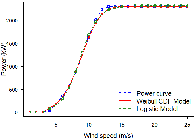
x <- fitcurve(da)
## Weibull CDF model
## -----------------
## P = 1 - exp[-(S/C)^k]
## where P -> Power and S -> Speed
##
## Shape (k) = 4.242446
## Scale (C) = 9.564993
## ===================================
##
## Logistic Function model
## -----------------------
## P = phi1/(1+exp((phi2-S)/phi3))
## where P -> Power and S -> Speed
##
## phi 1 = 2318.242
## phi 2 = 8.658611
## phi 3 = 1.366054
## ===================================
x
## $Speed
## [1] 1 2 3 4 5 6 7 8 9 10 11 12 13 14 15 16 17 18 19 20 21 22 23 24 25
##
## $Power
## [1] 0 0 0 35 175 352 580 870 1237 1623 2012 2230 2300 2300 2300
## [16] 2300 2300 2300 2300 2300 2300 2300 2300 2300 2300
##
## $`Weibull CDF`
## [1] 0.0000 0.0000 0.0000 90.3871 175.0000 327.5161 563.9085
## [8] 882.3965 1253.7489 1623.0000 1929.1254 2134.6685 2242.6251 2285.2438
## [15] 2297.3355 2299.6816 2299.9764 2299.9990 2300.0000 2300.0000 2300.0000
## [22] 2300.0000 2300.0000 2300.0000 2300.0000
##
## $`Logistic Function`
## [1] 0.00000 0.00000 0.00000 74.12834 148.99362 289.70750
## [7] 530.79747 884.98926 1303.20935 1686.50694 1964.36660 2133.40768
## [13] 2225.51217 2272.70001 2296.11395 2307.54706 2313.08621 2315.75963
## [19] 2317.04756 2317.66748 2317.96573 2318.10919 2318.17820 2318.21138
## [25] 2318.22734
##
## attr(,"class")
## [1] "fitcurve"
## attr(,"row.names")
## [1] 1 2 3 4 5 6 7 8 9 10 11 12 13 14 15 16 17 18 19 20 21 22 23 24 25
validate.curve(x)
## Metrics Weibull CDF Logistic Function
## 1 RMSE 30.8761687 38.8753476
## 2 MAE 15.1381094 29.3213877
## 3 MAPE 3.9292946 5.9183675
## 4 R2 0.9989322 0.9983073
## 5 COR 0.9995413 0.9991591
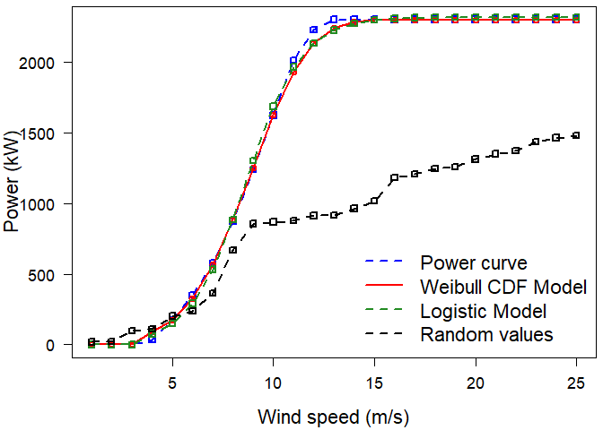
plot(x)

User can utilize
WindCurvespackage as a testbench so that a new curve fitting technique can be compared with above mentioned existing environment.- The user defined function (similar to
random()) should be saved in .R format and it should return the fitted values in terms of “Power values”. Therandom()function used in this example is stored as .R file withdump()function and made available in theWindCurvespackage and written as:
random <- function(x) { data_y <- sort(sample(1:1500, size = 25, replace = TRUE)) d <- data.frame(data_y) return(d) } dump(“random”) rm(random)
- The user defined function (similar to
- A
random()function is attached in the comparison the parametersMethodPathandMethodNameas shown below, whereMethodPathis a location of the function proposed by the user andMethodNameis a name given to the function.
#
library(WindCurves)
data(pcurves)
s <- pcurves$Speed
p <- pcurves$`Nordex N90`
da <- data.frame(s,p)
x <- fitcurve(data = da, MethodPath = "source('dumpdata.R')", MethodName = "Random values")

##    Weibull CDF model
##    -----------------
##    P = 1 - exp[-(S/C)^k]
##    where P -> Power and S -> Speed
##
##     Shape (k) = 4.242446
##     Scale (C) = 9.564993
##    ===================================
##
##    Logistic Function model
##    -----------------------
##    P = phi1/(1+exp((phi2-S)/phi3))
##    where P -> Power and S -> Speed
##
##     phi 1 = 2318.242
##     phi 2 = 8.658611
##     phi 3 = 1.366054
##    ===================================

## The user can specify .R files from other locations as:
# x <- fitcurve(data = da, MethodPath = "source('~/WindCurves/R/random.R')", MethodName = "Random values")
validate.curve(x)

##   Metrics Weibull CDF Logistic Function Random values
## 1    RMSE  30.8761687        38.8753476   865.0612001
## 2     MAE  15.1381094        29.3213877   722.4000000
## 3    MAPE   3.9292946         5.9183675    83.1646542
## 4      R2   0.9989322         0.9983073     0.1618424
## 5     COR   0.9995413         0.9991591     0.9487730

plot(x)
- Also,
WindCurvesallows user to add more error measures withvalidate.curve()function as explained below:
Consider error() is a function which uses two vectors as input and returns a error value with a specific error measure, such as RMSE or MAPE as shown below:
# PCV as an error metric
error <- function(a,b)
{
d <- (var(a) - var(b)) * 100/ var(a)
d <- as.numeric(d)
return(d)
}
dump("error")
rm(error)
The effect of this function can be seen in the results obtained with Validate.curve() function as:
library(WindCurves)
data(pcurves)
s <- pcurves$Speed
p <- pcurves$`Nordex N90`
da <- data.frame(s,p)
x <- fitcurve(da)

##    Weibull CDF model
##    -----------------
##    P = 1 - exp[-(S/C)^k]
##    where P -> Power and S -> Speed
##
##     Shape (k) = 4.242446
##     Scale (C) = 9.564993
##    ===================================
##
##    Logistic Function model
##    -----------------------
##    P = phi1/(1+exp((phi2-S)/phi3))
##    where P -> Power and S -> Speed
##
##     phi 1 = 2318.242
##     phi 2 = 8.658611
##     phi 3 = 1.366054
##    ===================================

validate.curve(x = x, MethodPath = "source('dumpdata.R')", MethodName = "New Error")

##     Metrics Weibull CDF Logistic Function
## 1      RMSE  30.8761687        38.8753476
## 2       MAE  15.1381094        29.3213877
## 3      MAPE   3.9292946         5.9183675
## 4        R2   0.9989322         0.9983073
## 5       COR   0.9995413         0.9991591
## 6 New Error  -1.8141636         0.4127417

plot(x)
Similarly, user can compare various techniques used for wind turbine power curve fitting.
- Dataset [2] on the power curves of wind turbine from four major manufacturers: Siemens, Vestas, REpower and Nordex. These datsset represent wind turbine power output in ‘kW’ against wind speed in ‘metres per second’ as shown below:
## data(pcurves) pcurves
##    Speed Vestad V80 Vestad V164 Siemens 82 Siemens 107 Repower 82 Nordex N90
## 1      1          0           0          0           0          0          0
## 2      2          0           0          0           0          0          0
## 3      3          0           0          0           0          0          0
## 4      4          2         101         42          80         64         35
## 5      5         97         461        136         238        159        175
## 6      6        255         902        276         474        314        352
## 7      7        459        1595        470         802        511        580
## 8      8        726        2513        727        1234        767        870
## 9      9       1004        3737       1043        1773       1096       1237
## 10    10       1330        4988       1394        2379       1439       1623
## 11    11       1627        5987       1738        2948       1700       2012
## 12    12       1772        6698       2015        3334       1912       2230
## 13    13       1797        6984       2183        3515       2000       2300
## 14    14       1802        6985       2260        3577       2040       2300
## 15    15       1802        6995       2288        3594       2050       2300
## 16    16       1802        6995       2297        3599       2050       2300
## 17    17       1802        6995       2299        3600       2050       2300
## 18    18       1802        6995       2300        3600       2050       2300
## 19    19       1802        6995       2300        3600       2050       2300
## 20    20       1802        6995       2300        3600       2050       2300
## 21    21       1802        6995       2300        3600       2050       2300
## 22    22       1802        6995       2300        3600       2050       2300
## 23    23       1802        6995       2300        3600       2050       2300
## 24    24       1800        6995       2300        3600       2050       2300
## 25    25       1800        6995       2300        3600       2050       2300
Further,
WindCurvespackage provides feature to extract/capture Speed Vs Power discrete points from power curve image. This can be achieved with the following simple instruction:#img2points(“image.jpeg”)
where, image.jpeg is the name of power curve image from which discrete points are to extracted. The procedure of extraction is as follows:
- With the command
img2points("image.jpeg"), an image will get appeared in the Viewer. - Click on leftmost point of the X-axis of the curve image and assign the respective appropriate value.
- click on rightmost point on X-axix, downmost point of Y-axis and topmost point of Y-axis, and assign their values, respectively.
- click of the points on the curve image. By default, 15 points can be captured from the curve image, but user can set the desired number of points with
nparameter inimg2points()function. - This function returns a data.frame with two columns, i.e., wind speed and wind power, which can be used as input data for
fitcurve()function.
References Permalink
[1] D. Villanueva and A. E. Feij´oo, “Reformulation of parameters of the logistic function applied to power curves of wind turbines,” Electric Power Systems Research, vol. 137, pp. 51–58, 2016.(via)
[2] Iain Staffell, “Wind turbine power curves, 2012” (via)